Published on February 22nd, 2025 | by David Marshall
0
Episode 163: Ecosystem Engineers
An ecosystem can be described as all the interactions that occur between organisms and their physical environment. The processes acting within an ecosystem operate on a wide range of spatial and temporal scales and include both biotic and abiotic factors.
Ecosystem engineers are those species that have a significant impact on the availability of resources to other species and can be responsible for the creation, maintenance, modification or destruction of an ecosystem. The introduction, or even removal, of such a species can have profound effects on both physical and biological elements of an ecosystem.
Whilst we can recognise the impact of ecosystem engineers in modern systems (e.g. the introduction of an invasive species), we don’t fully understand what happens when an entirely new ecosystem engineering behaviour evolves. This has undoubtedly happened numerous times throughout geological time with the Great Oxygenation Event and the Cambrian Substrate Revolution being notable examples.
Joining us for this episode is Dr Tom Smith, University of Oxford, who has been using a computational approach to try to model what happens when an ecosystem engineer is introduced into an environment. The open access study is available to read here.
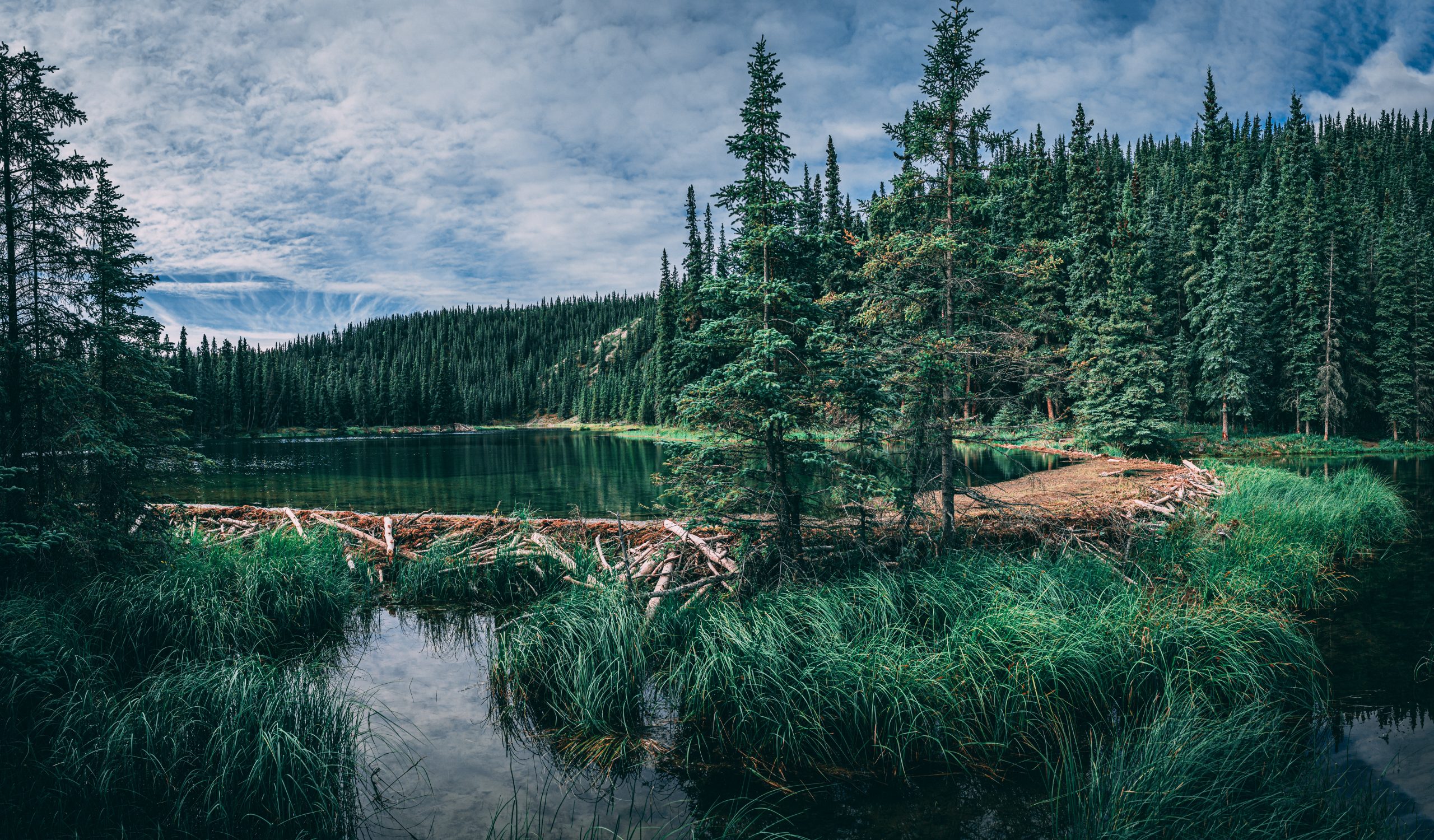
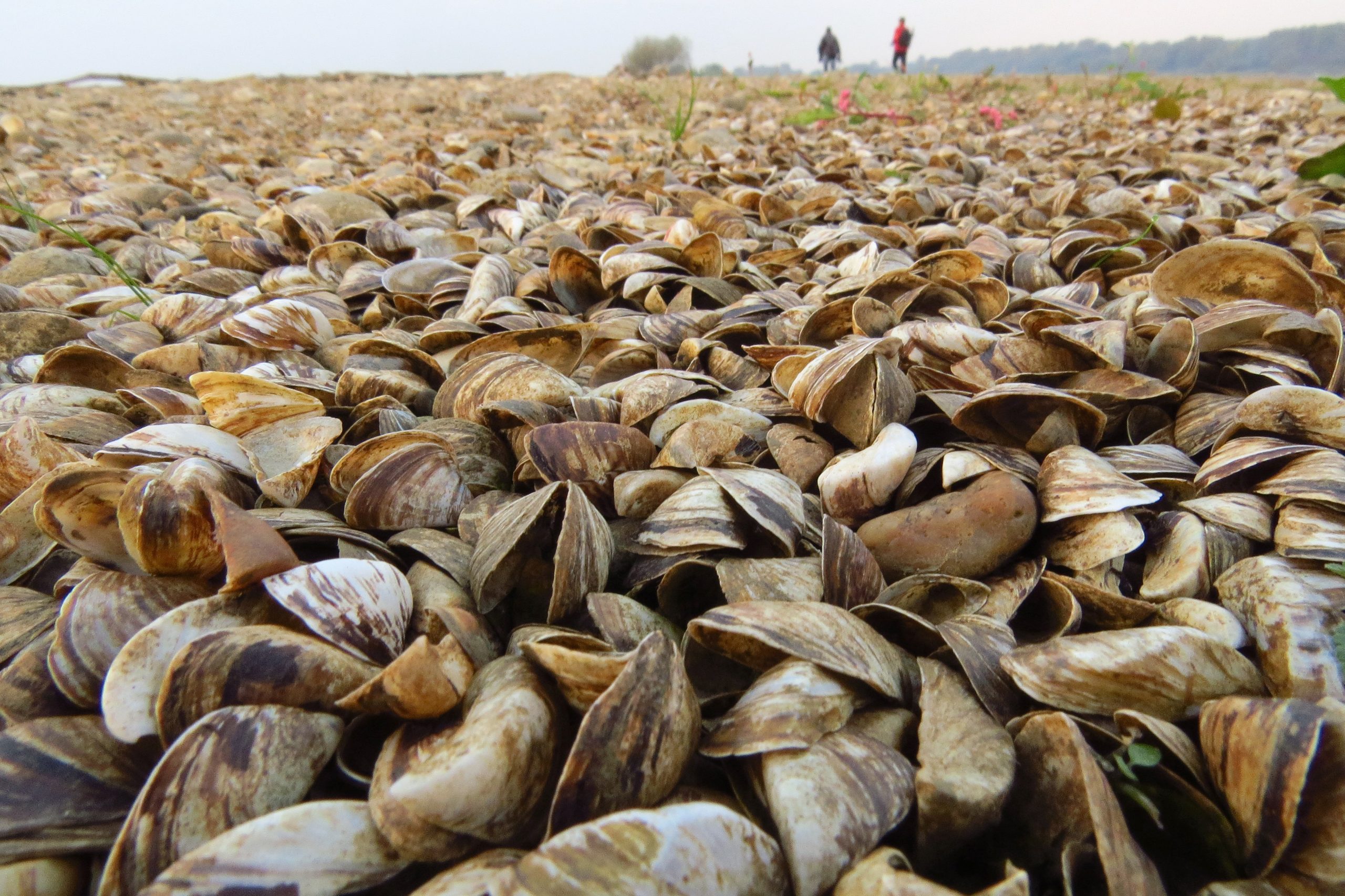
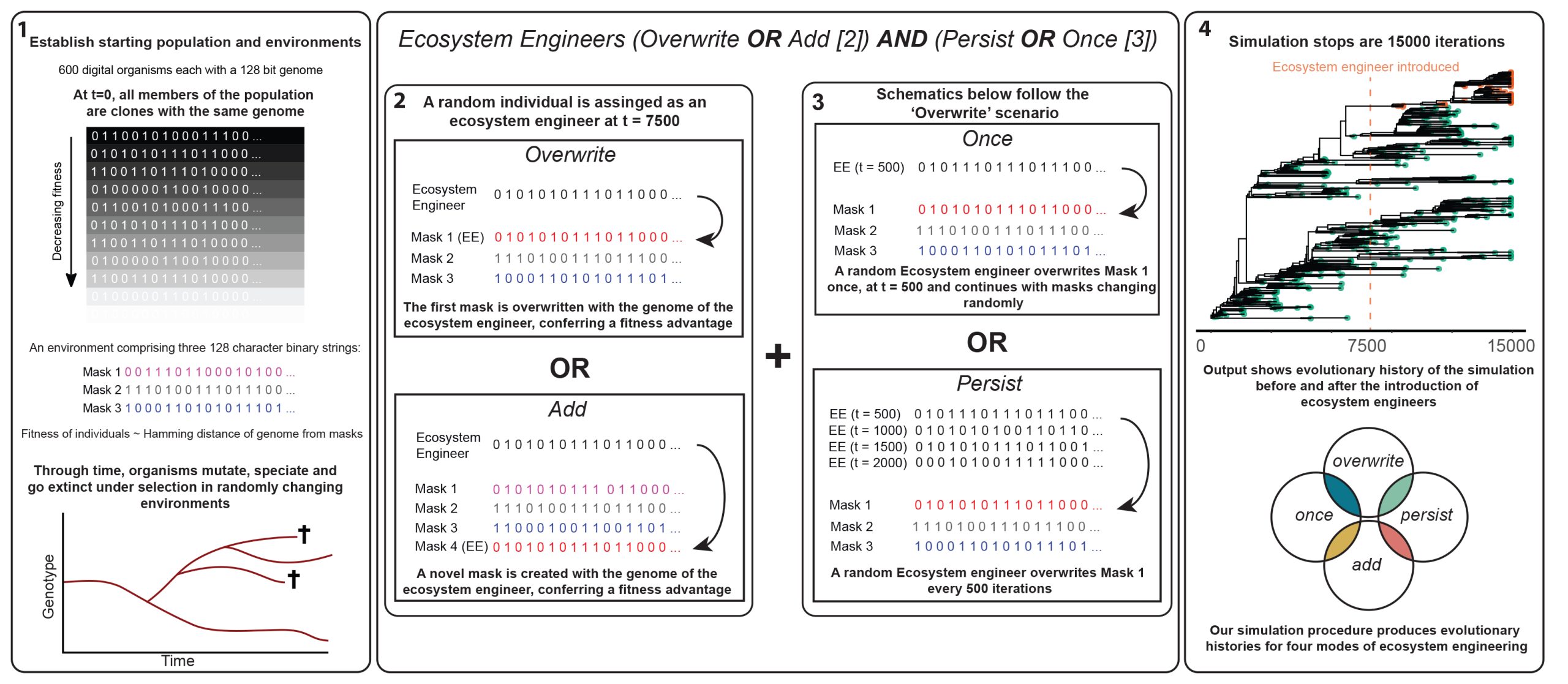
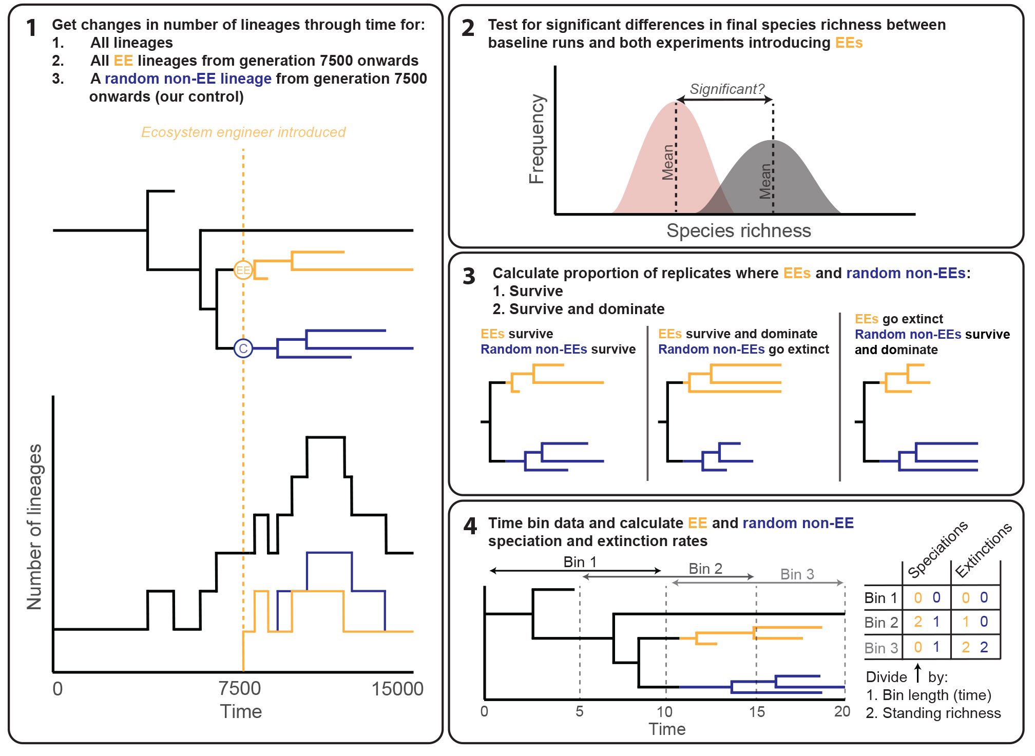
One of the most obvious examples of ecosystem engineering are beaver dams. In this case, it is the behaviour of an organism that has modified the physical environment and caused numerous trickle-down effects. Biotic systems may be affected through e.g. the creation or destruction of habitats, whilst abiotic systems such as e.g. oxygen availability or nutrient cycling are also altered. Image: Beaver dam in Horseshoe lake in Denali national park, Alaska.Ecosystem engineering can occur at different spatial and temporal scales and the Great Barrier Reef, Australia, is an example of an ecosystem that has been operating over a larger geographic area for a much longer time. Throughout geological history, reefs have been constructed by several different groups of organisms but regardless of whatever constructs them, the build-up of skeletal remains can have a profound impact on the environment. Today, the Great Barrier Reef is a hotspot for biodiversity, whilst fringe reefs, for example, can provide the shelter that mangrove forests need to grow.Ecosystem engineers can also upset or even destroy existing ecosystems with the invasive zebra mussels (Dreissena polymorpha) in the Great Lakes of North America being a good example. Zebra mussels can populate nearly any surface and can be so numerous that they smother native organisms. Furthermore, since these mussels are so good at filter feeding, they are able to drastically improve the water quality, removing sediment and pollutants. Cleaner waters allow light to penetrate further, which results in increased primary production and a restructuring of food webs.To investigate the impact of the introduction of a new ecosystem engineering behaviour, Dr Smith and colleagues devised a computational model. Here, the ‘genomes’ of digital ‘organisms’ were randomly created from a string of 128 binary numbers and placed within a digital ‘environment’ composed of three variables called ‘masks‘ (also a string of 128 binary numbers). The closer aligned the genomes of an organism were to the masks that made up their environment, the more likely they were to survive and reproduce. The evolution of these organisms was simulated 15,000 times over to quantify the range of outcomes. Once this baseline was established, the model was repeated under the following four scenarios, each of which introduced a different version of ecosystem engineering at the halfway point.
Simulation Scenarios
A random organism is selected to be an ecosystem engineer. The genome of this organism overwrites one of the 3 masks and the simulation runs to completion. This could represent the environment being altered by an organism.
A random organism is selected and its genome is added as a fourth mask and the simulation run to completion. This could represent an organism having adding extra complexity or ecospace to its environment.
A random organism is selected to overwrite a mask (the same as Scenario 1), but every 500 iterations the mask is overwritten by a randomly chosen descendent of the original ecosystem engineer. This means that the change persists throughout the simulation.
A random organism is selected to be added as a fourth mask (the same as Scenario 2), but the mask is updated with the genome of a randomly chosen descendent of the original ecosystem engineer every 500 iterations so that the change persists throughout the simulation.
The effect the ecosystem engineers had on the simulation under each of these scenarios was then recorded. By looking at the success of the different lineages through time, the researchers were able to examine the following.
Analysis
What was the relative success rate for ecosystem engineers (EEs) and non-ecosystem engineers (non-EEs) after the halfway point? This was determined by tallying the number of simulations in which the descendants of a species, be it an EE or non-EE, went extinct or survived until the end.
Did the introduction of an EE ultimately lead to an increase or decrease in species richness?
What is the likelihood that either group will go extinct (leading to the ‘domination’ by the other) or that both will survive?
What were the speciation and extinction rates through time?
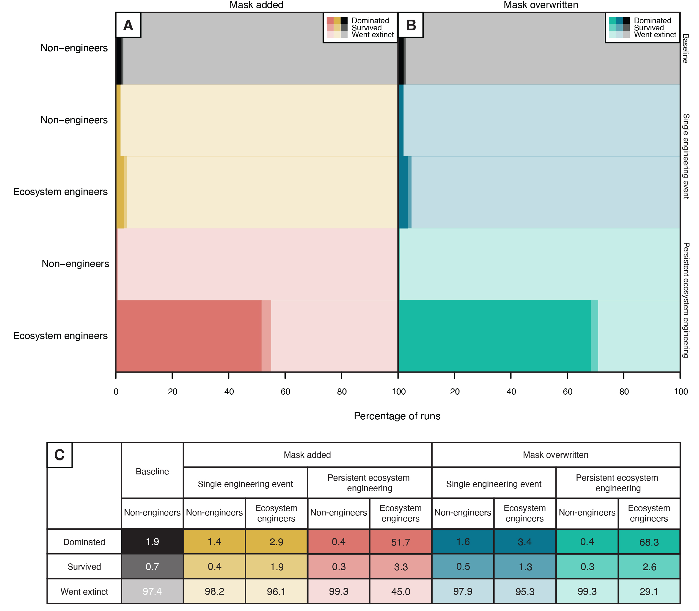
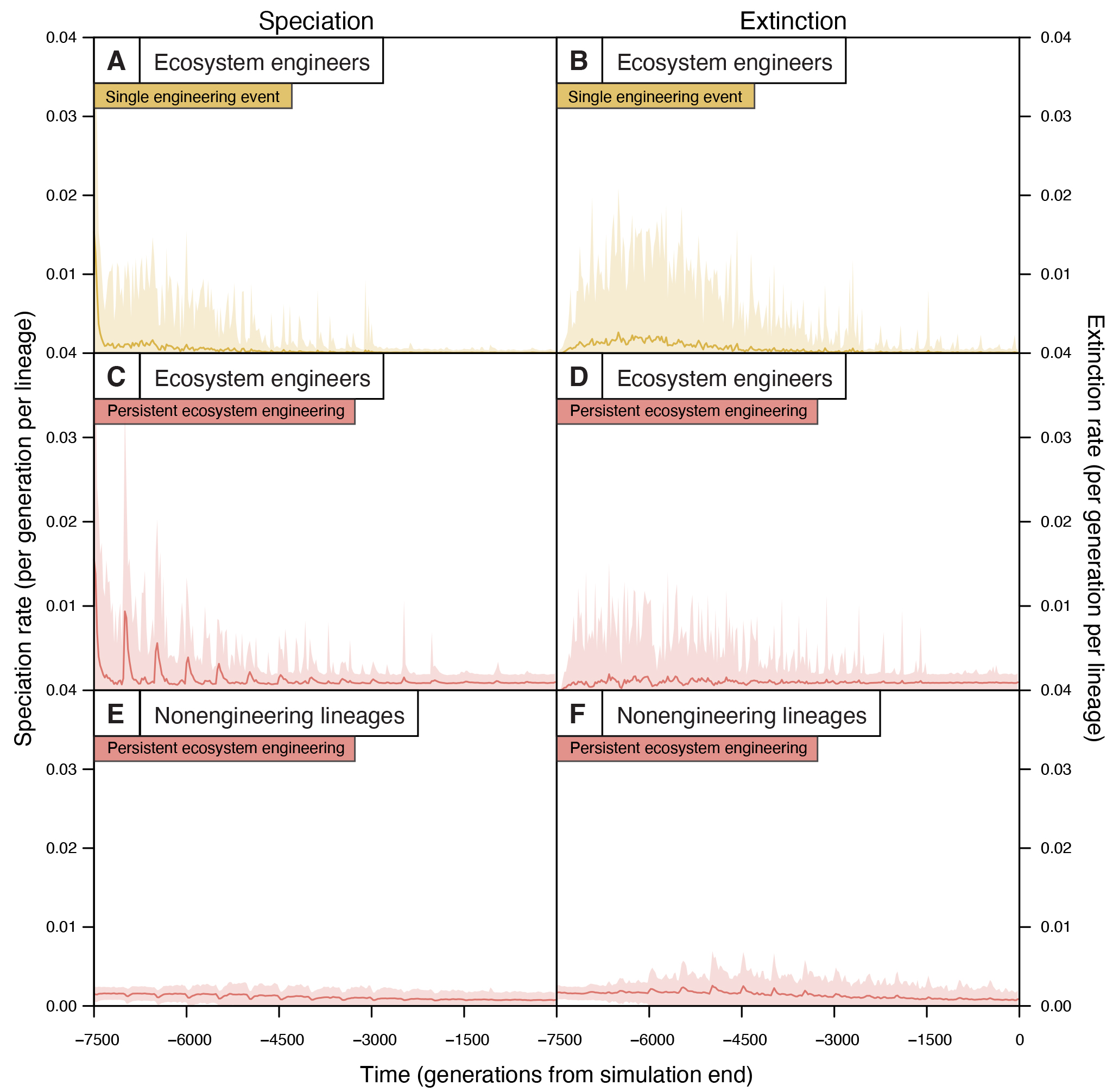
Whilst you might predict that EEs would likely go on to dominate most scenarios, their success was not guaranteed. In fact, it is only when persistent ecosystem engineering was introduced (red and green above) that the EEs would go on to dominate in over half of the simulations. Otherwise, in single events, EE lineages would eventually go extinct around 95 – 96% of the time (blue and yellow), faring only marginally better than the baseline expectation of 97.4% (black). Regardless of the scenario, any time a species was designated as an EE, that lineage showed improved survivability compared to non-EEs. Where an environmental mask was overwritten, as opposed to a new one being added, the impacts were much greater.The rates of speciation (left column) and extinction (right column) also provided interesting information. When an EE is introduced just once (A, B), the speciation rate of EEs immediately jumps before steadily falling, whereas the extinction rate for its descendants has a delayed response, gently peaking around 1000 iterations afterwards and steadily falling. Non-EEs (not-shown) show a flat rate of speciation and extinction bar small increases once the EE is introduced. When EEs are persistently introduced, there are peaks in speciation (C) and troughs in extinction (D) that decrease in magnitude with time following each event. Non-EEs show a corresponding dip in speciation (E) and peak in extinction (F) at each event.
These results not only show that ecosystem engineers exert an influence over their environments, they also possess a selective advantage that results in higher speciation and lower extinction rates. Even if the ecosystem engineering is a one-off event, the impacts in the short-term can be huge and whilst this instability lessens with time, the descendants of the ecosystem engineer will retain some selective advantage.
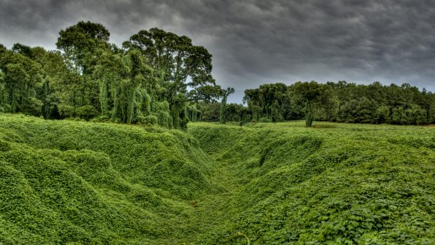
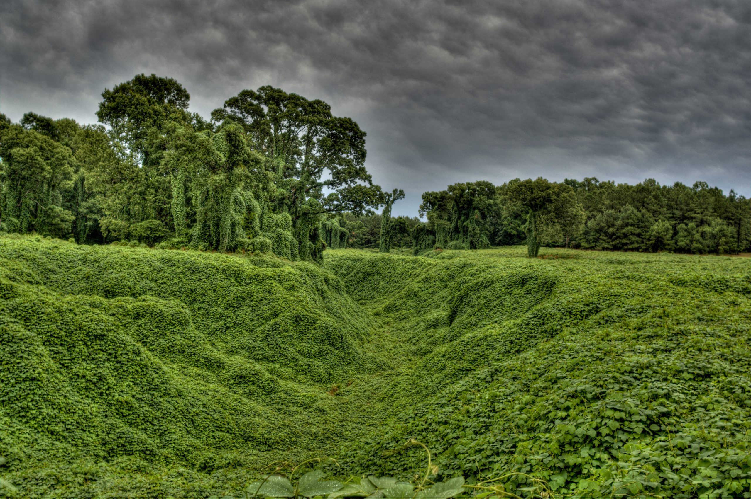
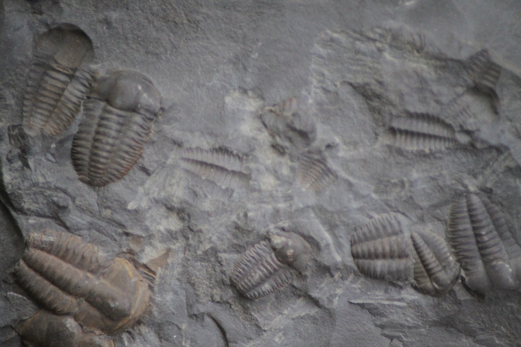
Understanding this, we are able to recognise that significant biological events in the past, such as the faunal turnover between the Ediacaran and Cambrian periods, could have been driven by the advent of new ecosystem engineering behaviours. Image credit: Carel Brest van Kempen.We are also able to apply these results to modern ecosystems and better understand that an invasive species can have a long-lasting impact on an ecosystem, even after it has disappeared. Image: Kudzu (Pueraria montana var. lobata), an invasive species to North America.
We are committed to creating the highest quality palaeontological multimedia with no advertisements and at no cost to our audience.
We are now using Patreon to allow us to give something extra back to all those who contribute to the improvement of our show. Please chck out our reward tiers below!
Thank you for anything you can give!